Unified Robotics III: Manipulation
Aug. 2018 – Oct. 2018
This is a team project with Michael Abadjiev and Nicholas Johnson.
This project was aimed at understanding the serial robot kinematics, trajectory generation and control as well as basic computer vision. The goal is to use camera to locate object and sort them by weight and color using a provided 3-DOF (degree of freedom) robot arm.
- Implemented a position controller for a 3-DoF robot arm with both forward and inverse kinematics.
- Created two inverse kinematics with either geometric close-form equations, and iterative method using Jacobian.
- Identified target objects and determined their position in the robot’s coordinate frame through computer vision.
- Weighted the object through holding torque from the robotic arm and sorted targets accordingly.
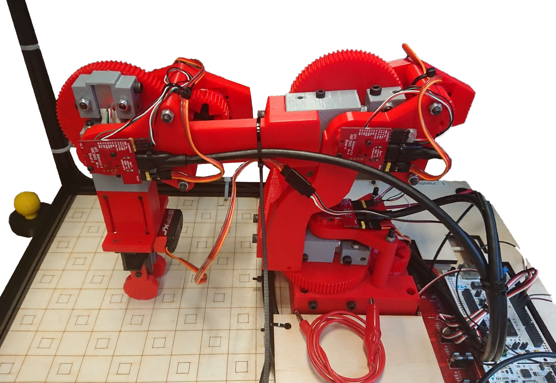
Provided 3-DOF robot arm with it's work area.
A video with top view of the robot in action sorting objects along with the kinematic stick plot in the corner.
The project uses MATLAB to handle all the math and high level controller. In addition, a 3D stick plot representing the robot kinematic is resented in real-time using MATLAB’s plot3.
To convert joint angle into the robot’s tool tip position, forward kinematics is the solution. Forward kinematics of this robot is obtained by combining the transform matrix between each joint’s coordinate frame. Each joints’ frame is determined using the DH-convention. To make the z-axis of the tool tip pointing away from it, according to the DH-convention, a phantom joint is used to flip the frame into the right configuration.
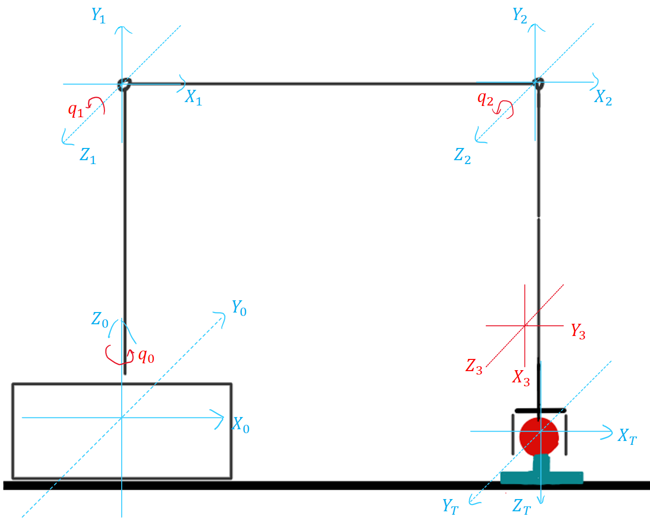
Transfer frame definition of the arm.
The figure above shows the frames and axis definition for the robot in X,Z view. Due to the limitation of DH nation, the frame {X3 Y3 Z3} in red color is the phantom joint to help achieve a +Z pointing out the end-effector.
The most common solution for solving the inverse kinematics of a serial robot is to use an iterative method based on Jacobian matrix. This is essentially simulating the robot’s motion using forward kinematics and guess for the correct inverse kinematics iteratively. Luckily, our robot is simple enough to have a geometric close form solution for the inverse kinematics. After implementing both approach and evaluated their performance. The fast and simple geometric solution is used.
The camera mounted on the robot’s base frame provided a way to use basic computer vision to locate objects. A picture of the field will be taken by the camera, then the color mask is used to isolate object of the specific color. With the help of some MATLAB function, any round object with the same size as the field object is located. This location is then transformed to robot’s tool space which robot can react on.
For a smooth motion, trajectory planning is necessary. A quantic polynomial is applied onto the robot’s future path for generating the trajectory of zero initial velocity, acceleration, and jerk. This resulting trajectory will then be convert into motion plan and sent to robot for its movement.