Rotary Stewart Platform Stabilizer Kinematics Design
June 2020 – August 2020, WPI
This is a team project with Michael Abadjiev.
- Designed the kinematics for a rotary stewart platform that uses servo motor instead of linear actuators.
- Created a unique close form equation for the inverse-kinematics of the stewart platform using frame transformation and vector geometries. This equation is adaptive to various kinds of platform configuration and servo mounting pattern.
- Visualized both rotation and translation workspace with robot’s parameters in MATLAB to finalize a optimal configuration.
- Simulated the kinematic model of the Stewart platform with basic controller through MATLAB.
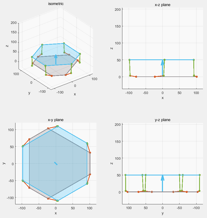
MATLAB simulation of the servo stabilization Stewart platform (gray is the moving base, blue is the stabilized platform)
Stewart platform is one of the most famous parallel robot design. Compare to serial robot, it has much smaller workspace while also being less demanding on the actuator. A small Stewart platform can have many application. Here we aimed for the camera stabilization as it is close to our daily life.
A classic Stewart platform is made from 6 prismatic leg powered by linear actuators. However, linear actuators are generally very expensive. A cheap one can be made from lead screw. however, in the case of camera stabilization, the actuator needs fast response and lead screw actuators are precise but slow. Although direct timing belt driven linear actuator is possible, there is actually an simpler and well known solution: crank arm.
The crank arm design break up each of the 6 “leg” made from linear actuators into 6 pairs of crank arm and fix length leg. The crank arm will only rotate in one plane while the fix length leg will have ball joints on both end and free to move around. There are already many school and hobbyist project using this low-cost design.
Close Form Equations Inverse Kinematics
The inverse kinematics for a classic Stewart platform with linear actuator is actually very easy. With the desire location of the platform given, the upper leg mounting point is known. The lower leg mounting point is fixed. Then the prismatic leg is fully defined by the vector from the lower mounting point to the upper mounting point. Extracting the joint variable “leg length” is quite easy.
On the other hand, the inverse kinematic for the crank arm design is not this straight forward. The prismatic leg (virtual leg) is replaced by a pair of crank arm and fixed leg. The crank arm, fixed leg, and the virtual leg (from classic configuration) are forming a triangle with all three sizes known. One would think using a simple trigonometry could find the crank arm angle. However, the upper mounting point is not in the same plane where crank arm would rotate. The angle in the triangle is not the same angle for the servo. The solution is to find the plane which the crank arm rotates on by frame transformation and project all components onto this plane. Then the problem becomes a simple trigonometry calculation.
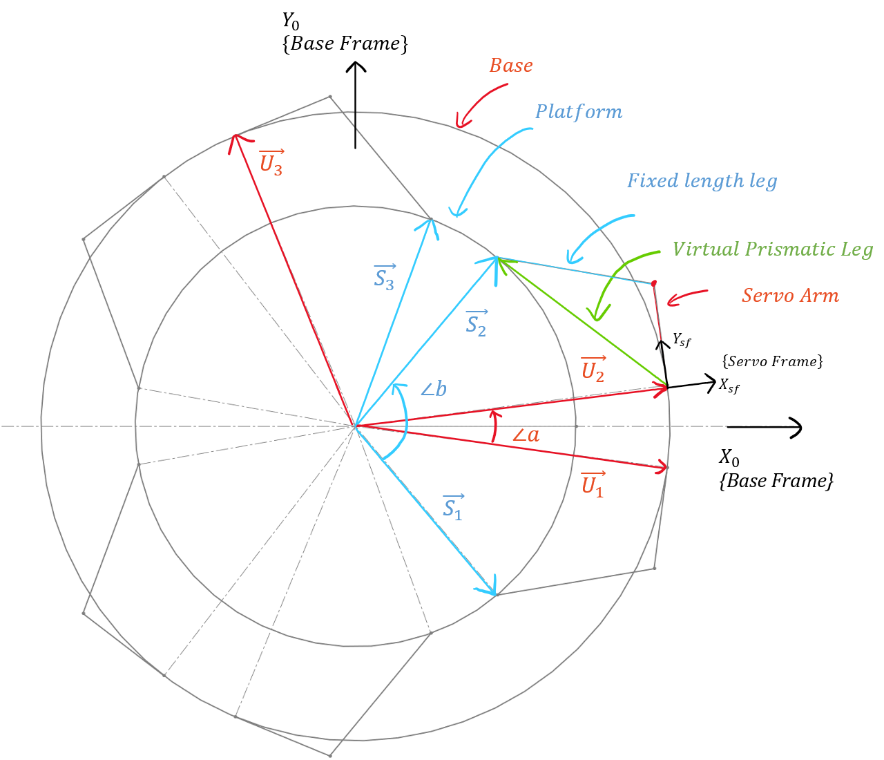
Top view of the servo Stewart platform kinematics
The image above showed a top view of an example crank arm Stewart platform kinematics. All the components are labeled in the graph. The first step to calculate joint angle for any leg is to generate the transformation frames of the servo where the projection will be based on. This transformation will consists of three steps. First, a rotation along the Z0 axis of the base frame to point X0 axis along the vector U. Second translate along the new X axis to reach the rotation center of the crank arm. Third, rotate along Z again to align the Xsf axis perpendicular to the plane of crank arm rotation.
Note how the Xsf axis in the servo frame is aligned with origin (with vector U). The rotation in third step to generate the servo frame will take into account of where the servo is pointing at. and the derived equation will work regardless of this alignment ( I have not tested the case of misalignment. While the plane is not perpendicular to vector U, it should be projected before being used by some of the math).
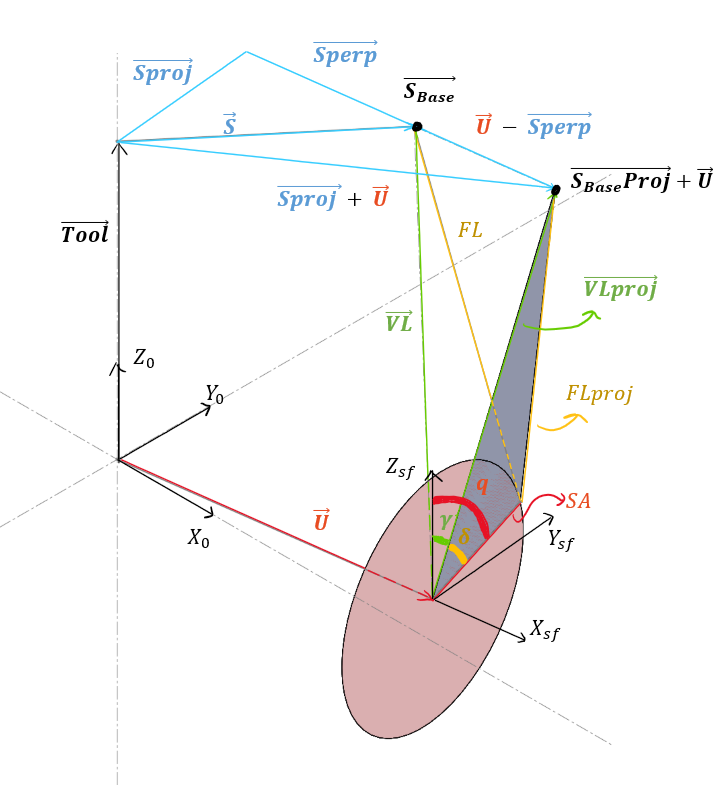
Kinematics of one leg with vector projection labeled.
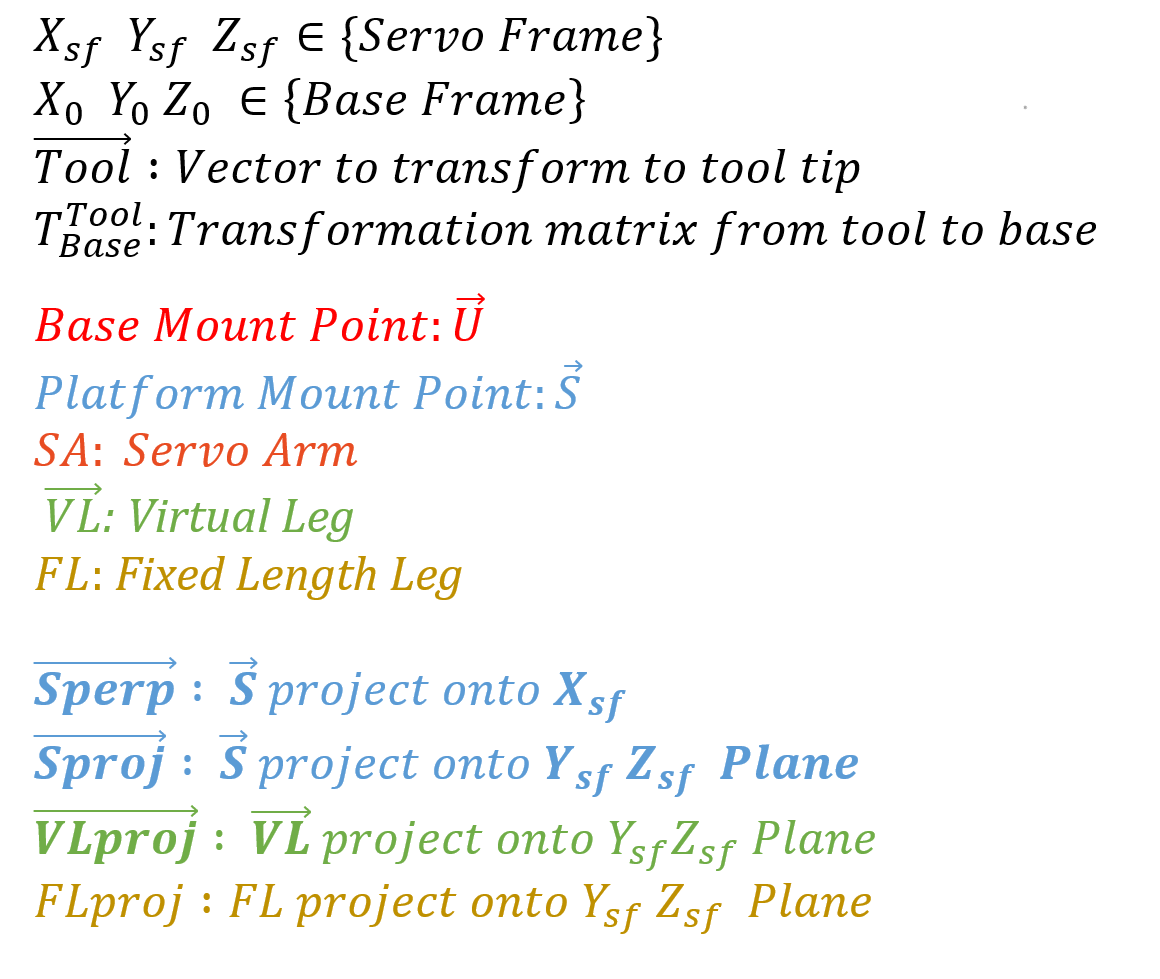
List of variables from within the drawing.
The image above showed the projection process and the components after projection. The Equation below shows the projection process and steps to find the length of both fixed leg and virtual leg after projection. Vector S is actually using the tool tip location as origin. The math needs to use vector SBase which includes the tool tip vector. However, for a clean illustration, the drawing above only shows vector S and its projection. Correspondingly, the first four equation below is done with vector S to match up with the graph. However, they are not mathematically correct, the lower four equations are.
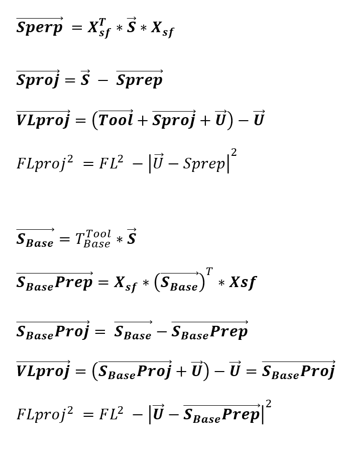
Equations for projection and finding length of both fixed and virtual leg after projection
Note: among the above equations top four are only for understanding, they are incomplete.
The tricky part is the length of fixed leg. The original fixed leg, projected fixed leg, and a section of the projected vector actually formed a right triangle in a different plane.
Combined the length of both leg after projection with the length of the servo arm, a triangle is established with all three sizes given. This triangle can then be used to find the joint angle. The exact steps are shown below.
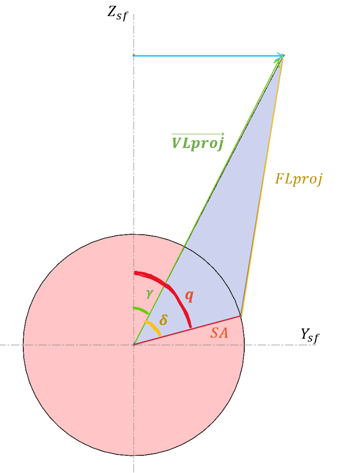
Side view of the servo plane with all the angles